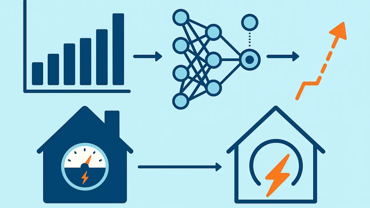
The model offers short-term energy demand forecasts for buildings and building assets for the next hours or days, with a granularity ranging from 15 minutes up to 1 hour in a time series format.
Energy consumption forecasting is performed using historical data collected at the asset level. Measurements are aggregated into hourly energy consumption values by default, with the option to increase granularity to 15-minute intervals if needed. Outlier values are detected and removed using the z-score method with a threshold of three standard deviations. To prepare the data for model training, min-max normalisation is applied to scale values between 0 and 1.
For training the model, a sliding window approach is used: each input sample includes the last 168 hours (one week) of consumption data, and the target output is the next hour’s consumption. A recurrent neural network based on gated recurrent units (GRUs) is used for prediction due to its simpler and faster-converging architecture compared to LSTM. The network has three GRU layers with 128, 64, and 32 units respectively, and includes dropout layers to reduce overfitting. The model is trained using an 80/20 training-validation split, with the Adam optimiser and mean squared error as the loss function.
The energy demand forecasting module provides hourly energy demand forecasts for the next 24 hours within a single building in a time series format through a REST API. In terms of initial modelling results, energy demand data from the RTU campus are utilised regarding assets within a single building. Specifically, electricity consumption from meter 4608 (2021/09/09–2024/10/28), which monitors room 209 on floor 2 of the Zunda 8 building, and from multiple HVAC assets. The metrics used for evaluation on the validation set are R2, mean squared error (MSE), and mean absolute error (MAE). After inversing the normalisation, the results were: MAE = 0.104 kWh, MSE = 0.158, and R2 = 0.8677. A model was also trained by aggregating the energy consumption of all the HVAC assets with the goal of predicting the total HVAC electricity demand of the building. After inversing the normalisation, the results were: MAE = 1.623 kWh, MSE = 9.356, and R2 = 0.883. In addition, a model was trained with energy data regarding room 209 on floor 2 of the Zunda 8 building. After inversing the normalisation, the results were: MAE = 0.117 kWh, MSE = 0.059, R2 = 0.69.
| Data | Description | Type | Unit | Temporal resolution | Spatial resolution |
| electricity consumption | metered electricity consumption of an asset | time series | kWh | 15 min or 1 hour | asset / building |
| outside temperature | temperature forecast from weather services | time series | °C | 1 hour | district |
| Data | Description | Input or output | Type | Unit | Temporal resolution | Spatial resolution |
| electricity consumption | electricity consumption forecast of an asset | output | time series | kWh | 15 min or 1 hour | asset / building |
Energy demand forecasts are used for demand response optimisation.
Τhe module was developed using Python (https://www.python.org/). In terms of libraries and frameworks, TensorFlow (https://www.tensorflow.org/) and Keras (https://keras.io/) were utilised for the deep learning model. After training, the model is saved as Pickle files or H5 files. NumPy (https://numpy.org/) and Pandas (https://pandas.pydata.org/) are adopted for data processing, such as data loading, resampling, cleaning, and time series manipulation. Scikit-learn (https://scikit-learn.org/stable/) is used for data normalisation (e.g. min-max scaling) and outlier removal (e.g. z-score). The Open-Meteo API (https://open-meteo.com/) and the Norwegian Meteorological Institute API (https://www.yr.no/en) are used to retrieve historical and forecasted weather data when needed.